Say you want to do some scientific computation like analyzing and visualizing a data set, doing some machine learning etc. You are not sure which approach will ultimately be successful, and as usual there will be some surprises in the data. The exploration of the data set still goes on while you are trying out different ways to process it. In these situations, feedback should be as quick as possible so you can build a solution in many small steps.
You also want to document your work, publish it on the web as HTML or PDF, maybe even make it reproducible. The documentation will have to include graphics, some mathematical formulae, or a table.
Over the years, I have tried several software packages that would allow me to combine exploration, processing and documentation. Here is a list of options, with my opinions about them.
LaTeX
LaTeX is a system for preparing documents with advanced typesetting (articles and books with a lot of math in them, for example). So as a standalone tool, LaTeX is only useful for writing up a report after the work is done. However, there are tools such as knitR and SWeave that let you inject the output of a computation into the document, see below.
Creating PDFs with lots of math is no problem, after all TeX (the basis of LaTeX) was created for typesetting printed books and articles. Writing raw LaTeX “source code” is quite different from what you’re used to in a word processor, so I recommend you use LyX to make authoring easier. There are several options for converting LaTeX to HTML. When I did LaTeX to HTML conversion several years ago, the available packages were really hard to install, or the HTML output was not easily configurable.
Emacs Org mode
As the Emacs Org mode home page says, “Org mode is for keeping notes, maintaining TODO lists, planning projects, and authoring documents with a fast and effective plain-text system.” The plain text is what you see in Emacs, but Org mode makes it easy to add headings, bullet lists, hyperlinks and even mathematical formulae (using LaTeX notation).
Among Org mode’s many features is a way to mix executable source code with prose, called Babel. The source code can be in python, R, ruby and many other languages. Output is shown in plain text, it may include tables. The output from one code snippet can be used as input to another code snippet (that may even be in a different language).
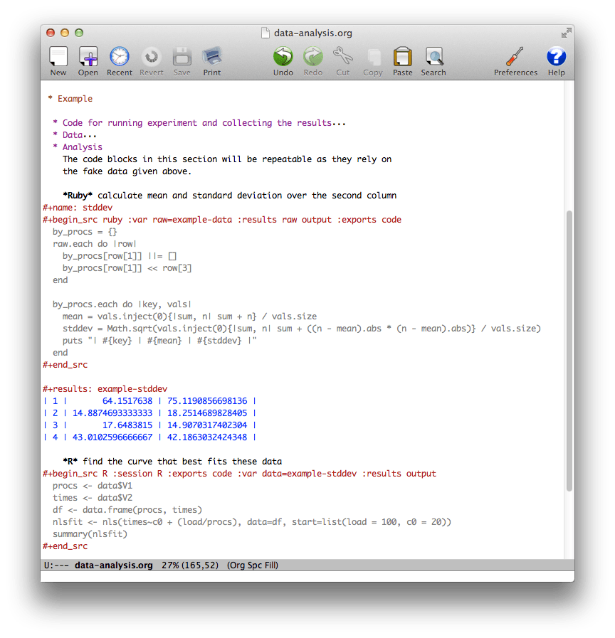
Example file from the Orgmode wiki
The org document can be exported to HTML and PDF (via LaTeX), with all computations executed before the export. That way, everything is re-computed so your document never goes out of sync with the computations.
The basic workflow is to write some explanations in plain text, add a code block, run it and see the result, all without leaving Emacs. You then edit the code block and re-run it until you are satisfied with the result. Then you move on to the next paragraph of explanations, some more code etc. The whole document can be exported and for each source code block you can decide if the code or only the output should be included.
Org mode can be used for reproducible research, see
Eric Schulte, Dan Davison, Thomas Dye, Carsten Dominik: A Multi-Language Computing Environment for Literate Programming and Reproducible Research Journal of Statistical Software, Vol. 46, Issue 3, Jan 2012
Re-running computations and waiting for the export to finish introduces some friction into the process. You have to match between the plain text source you edit and the resulting HTML (or PDF) which introduces some more friction.
Mathematica
Mathematica is a very fine computational system in many respects: programming language (symbolic, functional, procedural, pattern matching), graphical user interface (notebook interface with interactive graphics, math typesetting etc.), content (lots and lots of algorithms, including statistics, numerics, symbolic computation etc.). You can use Mathematica to produce PDF documents and HTML, I wrote my whole thesis in it in 1999.
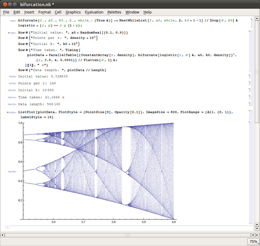
Image Credit: Wikipedia
A Mathematica notebook can combine formatted text (with headings, formulae, links etc) with computations and output in one document. When writing the document you build up a history of your work as well as documentation of the intermediate results. Feedback is immediate, you just re-evaluate one of the “input cells” that are interleaved with the explanatory “text cells”.
Recently I learned that Mathematica will be available for free on every Raspberry PI. I may want to buy one just to be able to run Mathematica on it.
MATLAB / Octave
I mention MATLAB here because it is very popular in engineering.
I have never worked with MATLAB or its open source clone GNU Octave.
I have been exposed to some MATLAB plotting commands through pyplot (see below).
From what I have seen so far, MATLAB’s programming language uses function names that are
quite hard to remember,
e.g. numel for the number of array elememts (array size).
Sage
Sage is a combination of different tools, many of them for symbolic computation, glued together with python. The notebook interface is nice (it comes from IPython, see below), but overall I found it not very attractive to work with all these different libraries. That is not the fault of sage (or python), but a consequence of bundling so many other systems (Maxima etc.)
R
R is the most popular open source statistics package by far. I have used it in some projects, but never learned to like it due to its abbreviated names and quirky programming language. Its strength lies in the large range of packages for all kinds of statistical and visualization tasks. The ggplot2 package is excellent for producing publication quality graphics and visualizations of complex data sets.
With knitR or the older SWeave you can create one document that combines explanations with R code. The document can then be processed to execute the computations and insert results into the text.
Here is a short video that shows knitr being used with documents written in Markdown or LaTeX:
It is even possible to write the document in LaTeX using LyX and then use knitr to produce the PDF document.
Just as with Org mode above, there is some friction in the process due to the lag time between making a change and seeing its result in the document.
IPython notebook
This is the most attractive option, IMHO, if you don’t want to buy Mathematica. You write the computations in Python, with the help from a numerics library like NumPy. There are many python packages for applications, like scikit-learn for machine learning or pylot for plotting. The notebook interface lets you combine explanations, computations and graphics. Code in the notebook can come from different languages (including R, Octave and UNIX shell) and you can use results from one language as input for a script in another language.
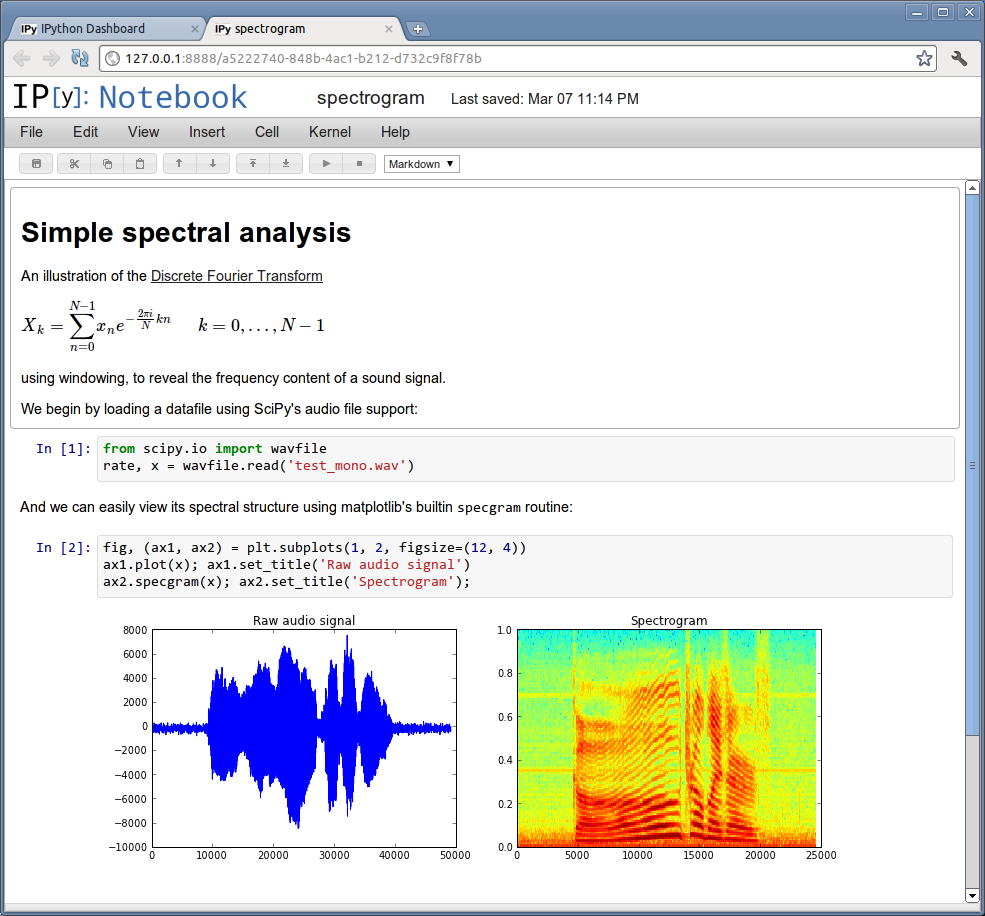
Image Credit: IPython development team
Using the IPython Notebook Viewer service you can publish the notebooks immediately on the web.
The most important thing is that you can build up a computation or an algorithm, explore your data, do several plots, all incrementally in one notebook, just like in Mathematica. The IPython notebook interface is heavily inspired by Mathematica and not yet as powerful. It also allows you to write and display formulae (using LaTeX syntax). The new nbconvert tool allows you to convert a notebook file to HTML, LaTeX, or a HTML slide show, among other formats.
I have used IPython notebook in several projects and I liked it. Especially the combination of IPython notebook and pandas is hard to beat when it comes to interactive data analysis.
Summary
Use IPython notebook if you want a free solution with good graphics, lots of libraries and a high level of interactivity. Access R from IPython if pandas is not enough for your analysis needs.
Use Mathematica if you want a well-integrated system with a very high level of interactivity and support for explorative analysis.
Use a combination of knitR and R or another scripting language if you want to produce standardized analysis reports for different data sets.